Gaussian-noise Linear Regression vs Multivariate Normal

We will discuss the creation of generative statistical models. For the purposes of demonstration, we’ll use the California housing dataset taken from scikit-learn. “The target variable is the median house value for California districts, expressed in hundreds of thousands of dollars” (8.2. Real world datasets). This dataset has been chosen simply because the target variable is continuous, making it capable of being predicted with linear regression, which is one of the models that we’ll be exploring. The other is the Multivariate Normal distribution.

from scipy.stats import fit, norm
from scipy.stats import multivariate_normal
from sklearn.datasets import fetch_california_housing
from sklearn.linear_model import LinearRegression
from sklearn.metrics import mean_squared_error
import matplotlib.pyplot as plt
import numpy as np
import pandas as pd
import random

random.seed(1)

data = fetch_california_housing()
attribute_names = [
    'Median Income',
    'House Age',
    'Average Rooms',
    'Average Bedrooms',
    'Population',
    'Average Occupation',
    'Latitude',
    'Longitude'
]

It is possible that not all of the variables belong to Gaussian distributions. Let’s plot their histograms overlayed with their respective Gaussian distributions to verify this hunch.

for i, col in enumerate(data.data.T):
    mu, sigma = np.mean(col), np.std(col)
    x = np.linspace(min(col), max(col), 200)
    plt.hist(col, bins=30, density=True)
    plt.xlabel(attribute_names[i])
    plt.plot(x, norm.pdf(x, mu, sigma))
    plt.show()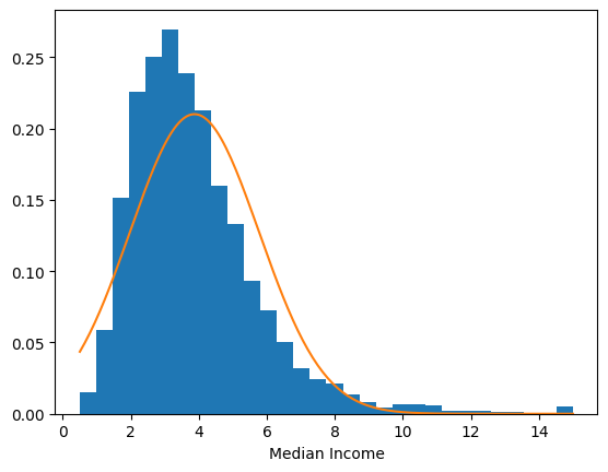

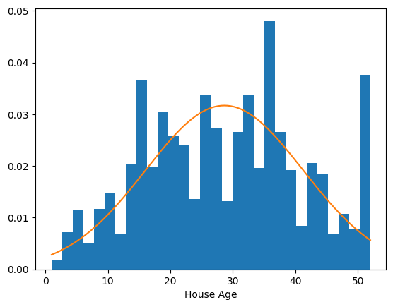
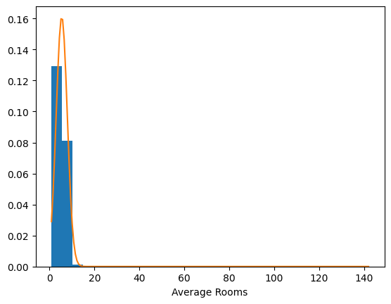
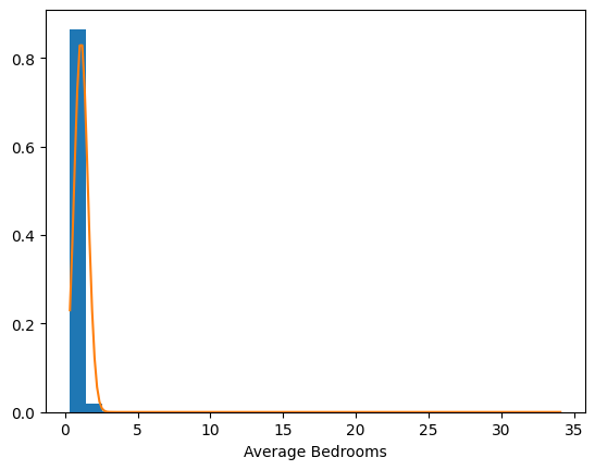
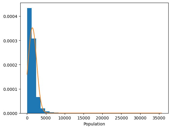
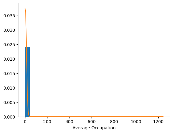
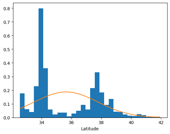
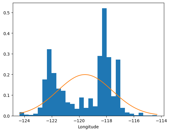
The distribution of longitude, for one, clearly does not follow a Gaussian distribution. Though different distributions might better serve us here, let’s keep things simple for now by assuming a multivariate Normal distribution for the X.

Of course, the fact that further refinement is possible (i.e., the employment of a multimodal distribution) has been noted for the sake of future work.

What about the target variable? What does that distribution look like?

mu, sigma = np.mean(data.target), np.std(data.target)
x = np.linspace(min(data.target), max(data.target), 200)
plt.hist(data.target, bins=30, density=True)
plt.plot(x, norm.pdf(x, mu, sigma))
plt.show()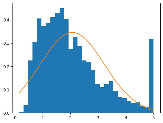

A Gaussian curve is not exactly flattering when worn by this variable. It is close enough, however, for our purposes in this article. In future work, I would like to experiment with other types of distributions.

Linear regression is defined as

We want this to not simply be a linear regression model, but a generative model, i.e., a Gaussian-noise linear regression model. (The noise is the $\epsilon$). When sampling from this model, we therefore sample the noise from the Gaussian distribution. The variance is

(Shalizi, 2017).

Depending on our data, we could sample the noise from any distribution where the expected value of $\epsilon$ is zero,

(Shalizi, 2017).

Below, we define our Gaussian-noise linear regression model. The sample method is what makes this model generative. We add noise to the samples because the observed data does not lay flat on a linear regression line. Rather, it expands outwards in a cloud that centers on the line. With noise introduced, therefore, the samples are more realistic.

# Gaussian noise linear regression model
class GaussianLinearRegression:
    def __init__(self, X, y):
        self.mu, self.cov = multivariate_normal.fit(X)
        self.lin_reg = LinearRegression()
        self.lin_reg.fit(X, y)
        y_pred = self.lin_reg.predict(X)
        self.sd = np.sqrt(mean_squared_error(y, y_pred))
        
    def sample(self, size=1):
        """
        Randomly sample from the probability distribution
        """
        X = multivariate_normal(self.mu, self.cov).rvs(size=size)
        if size == 1:
            X = X.reshape(1, -1)
        loc = self.lin_reg.predict(X)
        sample = norm(loc=loc, scale=self.sd).rvs(size=size)
        return np.append(X, sample)
    
    def log_likelihood(self, X, y):
        log_px = multivariate_normal(self.mu, self.cov).logpdf(X).sum()
        y_pred = self.lin_reg.predict(X)
        log_py_given_x = norm(loc=y_pred, scale=self.sd).logpdf(y).sum()
        return log_px + log_py_given_x
    
    def pdf(self, X, y):
        y_pred = self.lin_reg.predict(X)
        return norm(loc=y_pred, scale=self.sd).pdf(y)

glr = GaussianLinearRegression(data.data, data.target)
glr.sample()

array([ 1.65427924e+00, 1.64418672e+01, 6.12191566e+00, 1.33692717e+00, 1.38043401e+03, 1.09108617e+01, 3.56291888e+01, -1.18543129e+02, 8.78771712e-01])

I want to dwell a moment on the above implementation of log_likelihood. Log-likelihood is a measure of the goodness-of-fit (Taboga).

We can use it to compare the goodness-of-fit of one statistical model to the goodness-of-fit of another.

glr.log_likelihood(X=data.data, y=data.target)

-503782.5946747418

For our purposes pdf result that is closer to 0 is more 👎. A logarithm tends to negative infinity as the input tends towards 0. Therefore, a lower logpdf can be thought of as a comparatively more unlikely value. To demonstrate:

temp = norm(loc=0, scale=1)
temp.pdf(-1), temp.pdf(0), temp.pdf(1), temp.pdf(100), temp.logpdf(-1), temp.logpdf(0), temp.logpdf(1), temp.logpdf(100)

(0.24197072451914337, 0.3989422804014327, 0.24197072451914337, 0.0, -1.4189385332046727, -0.9189385332046727, -1.4189385332046727, -5000.918938533205)

The PDF is the probability density function. Because the probability of a continuous random variable taking on any value is 0, we use the PDF.

Because logarithms have the property that $\log(a b) = \log(a) \log(b)$, we summed their results to attain the log-likelihood.

def create_X_y(data):
    return np.append(data.data.T, [data.target], axis=0).T
X_y = create_X_y(data)
print('Shape of X_y', X_y.shape)
mu, cov = multivariate_normal.fit(X_y)
multivariate_normal(mu, cov).logpdf(X_y).sum()

Shape of X_y (20640, 9)

-503782.5946747417

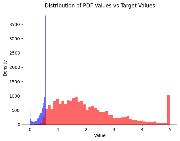
**The Gaussian-noise linear Multivariate Normal Simply because the target is not a linear function of the input.

We’ll show that to be the case by visually comparing the distribution of the target variable and the model’s guess for that target variable.

#plt.figure()
plt.hist(glr.pdf(data.data, data.target), bins=50, alpha=0.6, color='blue')

plt.hist(data.target, bins=50, alpha=0.6, color='red')

plt.xlabel('Value')
plt.ylabel('Density')
plt.title('Distribution of PDF Values vs Target Values')
plt.show()

If our ultimate goal were to build a model that accurately describes the data, then we would need to do better than our GaussianLinearRegression. Let’s also randomly sample from the model to compare that to the actual distribution.

sample = glr.sample(len(data.target))
plt.hist(sample, bins=50, alpha=0.6, color='blue')
plt.hist(data.target, bins=50, alpha=0.6, color='red')
plt.xlabel('Value')
plt.ylabel('Density')
plt.title('Distribution of PDF Values vs Target Values')
plt.show()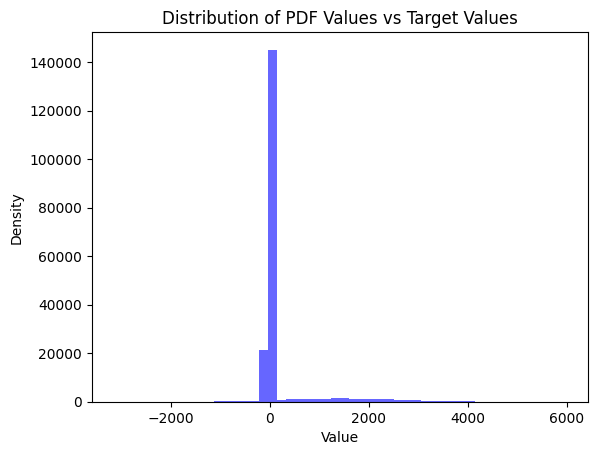

That doesn’t look like the same distribution to me.

The goodness-of-fit of the Gaussian-noise linear regression model is no better than that of the Multivariate Normal model.

In that case, why use it? Sure, you can use the former to predict y | X, but you can also do that with with the Multivariate Normal model. Doing so requires more code than what we’ve written, but not that much more.

In my opinion, if you’re trying to create a model that can generate, evaluate the pdf of an observation, and predict, then it’s a toss up between the two models. In a future post, we’ll be looking at other means of doing the same that also happen to fit the data more faithfully.

Bibliography

“8.2. Real World Datasets.” Scikit-Learn, https://scikit-learn/stable/datasets/real_world.html. Accessed 10 Feb. 2026.

Shalizi, Cosma. 36-401 Modern Regression, Fall 2017. 2017, https://www.stat.cmu.edu/~larry/=stat401/lecture-04.pdf.

Taboga, Marco. Model Selection Criteria. https://www.statlect.com/fundamentals-of-statistics/model-selection-criteria. Accessed 11 Feb. 2026.