Implementing Linear Regression from Scratch in Python to Understand How It Works

Published: 2026-01-24
Updated: 2026-01-24

First, let’s use the built-in Scikit-Learn. We’ll use the California Housing dataset as that is listed in the documentation as a “regression” dataset.

from sklearn.datasets import fetch_california_housing
from sklearn.linear_model import LinearRegression
from sklearn.metrics import r2_score
from sklearn.model_selection import train_test_split
import matplotlib.pyplot as plt
import numpy as np
import pandas as pd

df = fetch_california_housing(as_frame=True)
X = df.data
y = df.target
np.random.seed(0)
X_train, X_test, y_train, y_test = train_test_split(X, y, test_size=0.2)
X_train.head(), y_train.head()

( MedInc HouseAge AveRooms AveBedrms Population AveOccup Latitude \ 12069 4.2386 6.0 7.723077 1.169231 228.0 3.507692 33.83
15925 4.3898 52.0 5.326622 1.100671 1485.0 3.322148 37.73
11162 3.9333 26.0 4.668478 1.046196 1022.0 2.777174 33.83
4904 1.4653 38.0 3.383495 1.009709 749.0 3.635922 34.01
4683 3.1765 52.0 4.119792 1.043403 1135.0 1.970486 34.08

Longitude
12069 -117.55
15925 -122.44
11162 -118.00
4904 -118.26
4683 -118.36 , 12069 5.00001 15925 2.70000 11162 1.96100 4904 1.18800 4683 2.25000 Name: MedHouseVal, dtype: float64)

What is r2_score? It’s typically written as: $R ^ 2$ Pronounced “R-squared”, the coefficient of determination measures what proportion of the target variable is predicted by the model. It ranges from 0 to 1 and is sometimes stated as a percentage.

model = LinearRegression()
model.fit(X_train, y_train)
print("TRAIN:")
print(r2_score(y_true=y_train, y_pred=model.predict(X_train)))
print("")
print("TEST:")
r2_score(y_true=y_test, y_pred=model.predict(X_test))

TRAIN: 0.6088968118672871

TEST:

0.5943232652466202

def model(column: str):
    model = LinearRegression()
    X_train_subset = X_train[[column]]
    model.fit(X_train_subset, y_train)
    train_score = r2_score(y_true=y_train, y_pred=model.predict(X_train_subset))
    test_score = r2_score(y_true=y_test, y_pred=model.predict(X_test[[column]]))
    return train_score, test_score

for c in X_train.columns:
    print(model(c))

(0.47991412719941495, 0.4466846804895943) (0.01133589722637418, 0.010112709993501445) (0.023847425986299742, 0.019686674517510605) (0.0019727324864367013, 0.0026742213470939413) (0.0007318879607208784, -0.00022540672756665714) (0.0011001698651382785, -0.006489558238010673) (0.020363987996845134, 0.022215172774302072) (0.0022351265327293923, 0.0012984715729211782)

No single column has greater predictive power than using all of the columns together. However, we’re going to use the first column because that will make the math slightly easier.

class CustomLinearRegression:
    a_hat: float
    b_hat: float
    
    def train(self, X_train: np.array, y_train: np.array):

        y_summed = y_train.sum()
        X_dot_X = X_train.dot(X_train)
        X_summed = X_train.sum()
        X_dot_y = X_train.dot(y_train)

        n = len(X_train)
        self.a_hat = (y_summed * X_dot_X - X_summed * X_dot_y) / (n * X_dot_X - X_summed ** 2)
        
        self.b_hat = (n * X_dot_y - X_summed * y_summed) / (n * X_dot_X - X_summed ** 2)
    
    def predict(self, X: np.array):
        return X * self.a_hat + self.b_hat

model = CustomLinearRegression()
X_train_subset = X_train.iloc[:, 0].to_numpy()
y_train_array = y_train.to_numpy()
model.train(X_train=X_train_subset, y_train=y_train_array)

r2_score(y_true=y_train, y_pred=model.predict(X_train_subset))

y_pred = model.predict(X_train_subset)
print(r2_score(y_true=y_train_array, y_pred=y_pred))
print("TRAIN:")
print(r2_score(y_true=y_train_array, y_pred=model.predict(X_train_subset)))
print("")
print("TEST:")
X_test_subset = X_test.iloc[:, 0].to_numpy()
r2_score(y_true=y_test, y_pred=model.predict(X_test_subset))

0.4752542635984037 TRAIN: 0.4752542635984037

TEST:

0.43971655102712115

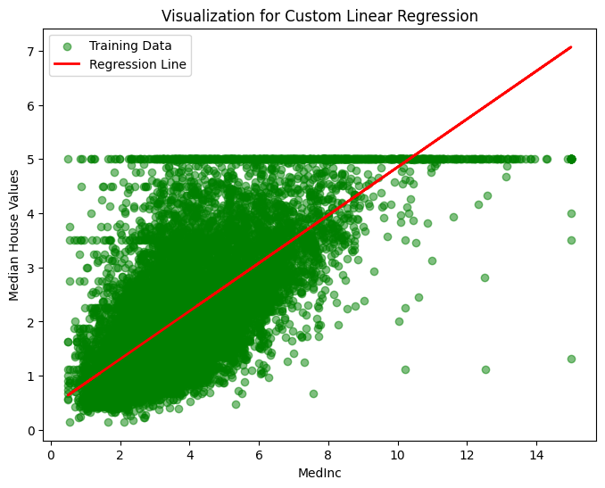
To end, let’s visualize the performance of the custom linear regresion model on the training data, because visualization give me the warm fuzzies.

plt.figure(figsize=(8, 6))
plt.scatter(X_train_subset, y_train, color='green', alpha=0.5, label='Training Data')
plt.plot(X_train_subset, y_pred, color='red', linewidth=2, label='Regression Line')
plt.title('Visualization for Custom Linear Regression')
plt.xlabel('MedInc')
plt.ylabel('Median House Values')
plt.legend()
plt.show()

A scatter plot showing a line of best fit

In just a few lines of code, we got a score that is similar to what we achieved with the SciKit-Learn implementation.

So what happened? Consider the following formula in which the training data, the estimated coefficients, and the target are terms.

\begin{bmatrix} n & \sum_{i=1}^n x_i \\[1ex] \sum_{i=1}^n x_i & \sum_{i=1}^n x_i^2 \end{bmatrix} \begin{bmatrix} \widehat{\alpha} \\[1ex] \widehat{\beta} \end{bmatrix} = \begin{bmatrix} \sum_{i=1}^n y_i \\[1ex] \sum_{i=1}^n y_i x_i \end{bmatrix}

From the previous can be derived the below. Conveniently, the coefficients to be estimated are isolated on the left-side.

\begin{align} \widehat{\alpha} &= \frac{ \left(\sum_{i=1}^n y_i\right)\left(\sum_{i=1}^n x_i^2\right) - \left(\sum_{i=1}^n x_i\right)\left(\sum_{i=1}^n x_i y_i\right) }{ n \sum_{i=1}^n x_i^2 - \left(\sum_{i=1}^n x_i\right)^2 } \\[8pt] \widehat{\beta} &= \frac{ n \sum_{i=1}^n x_i y_i - \left(\sum_{i=1}^n x_i\right)\left(\sum_{i=1}^n y_i\right) }{ n \sum_{i=1}^n x_i^2 - \left(\sum_{i=1}^n x_i\right)^2 }. \end{align}

(Wikipedia)

Unlike other paradigms (e.g., neural networks), a linear regression model is one that can be derived from the data analytically in a reasonable amount of time.

This model can also be interpreted in an intuitive way. After all, it’s just a line running through the two variables, signifying their correlation, and it comes pre-packaged with a measure of how far the data is from the line on average. We’re going to take advantage of this characteristic in a future post.