Linear Regression with PyMC
Performing Linear Regression with PyMC
A probabilistic way to estimate a linear relationship between two variables.
PyMC is library for probabilistic modeling. Here’s a brief primer on the terminology used herein:
-
“posterior” refers to the variable that is being modeled, i.e., the target or dependent variable.
-
“Markov Chain Monte Carlo” (MCMC) refers to a class of algorithms, the purpose of which is sampling from a probability distribution.
# Import scikit-learn modules, scipy, and numpy
from pprint import pprint
from sklearn import datasets, ensemble, feature_selection, preprocessing, linear_model
from sklearn.metrics import accuracy_score
from sklearn.metrics import confusion_matrix, classification_report
from sklearn.model_selection import train_test_split
import arviz as az
import graphviz
import matplotlib.pyplot as plt
import numpy as np
import pandas as pd
import pymc as pm

# Set the random seed/state for reproducibility
random_seed = 42
np.random.seed(random_seed)
Load the diabetes dataset from scikit-learn
From the Scikit-Learn documentation:
Number of Instances: 442
Number of Attributes: First 10 columns are numeric predictive values
Target: Column 11 is a quantitative measure of disease progression one year after baseline
Attribute Information: age age in years
sex
bmi body mass index
bp average blood pressure
s1 tc, total serum cholesterol
s2 ldl, low-density lipoproteins
s3 hdl, high-density lipoproteins
s4 tch, total cholesterol / HDL
s5 ltg, possibly log of serum triglycerides level
s6 glu, blood sugar level
The target variable is a quantitative measure of diabetes progression. https://scikit-learn.org/stable/datasets/toy_dataset.html#diabetes-dataset
X, y = datasets.load_diabetes(return_X_y=True)

# Scale the dataset to improve the accuracy of the logistic regression classifier
scaler = preprocessing.StandardScaler()
X = scaler.fit_transform(X)

X_train, X_validation, y_train, y_validation = train_test_split(X, y, test_size=0.2)

# Calculate the mean and standard deviation of y for setting priors
y_mean = np.mean(y_train)
y_std_dev = np.std(y_train)
print(f"mean of y is {y_mean}")
print(f"Std dev of y is {y_std_dev}")
print(f"Std dev of X:")
print(np.std(X_train, axis=0))
X_train[0], y_train[:5]
mean of y is 153.73654390934846
Std dev of y is 77.9512540821802
Std dev of X:
[0.97273717 1.0002379  0.99249697 1.01755207 1.0032151  0.99996932
 0.9876345  1.00330241 1.00410614 1.01569595]


(array([ 1.48782782,  1.06548848,  0.25474221,  1.18365854,  0.71913607,
         1.03891555, -0.83504852,  0.72130245,  0.57529619, -0.02265729]),
 array([144., 150., 280., 125.,  59.]))
# arvix won't display correctly if this isn't set
az.rcParams['plot.backend'] = 'matplotlib'
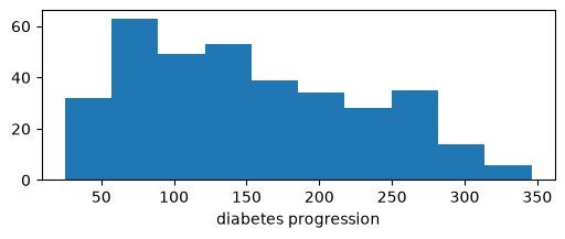
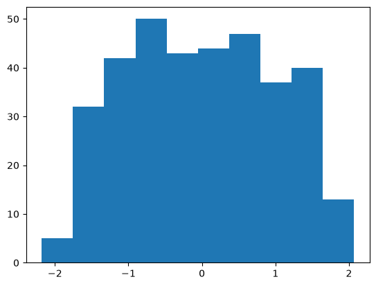
# Plot a histogram of the target variable
_, ax = plt.subplots(figsize=(6, 2))
_ = ax.hist(y_train, bins='auto')
plt.xlabel('diabetes progression')
plt.show()
In PyMC, we construct the computational graph of the model in a with block.
# Model y while ignoring the conditioning information
# Plot the Normal model
with pm.Model() as normal_model:

    # This variable can be set to different data later
    y = pm.Data('y', y_train)

    mu = pm.Normal('mu', mu=y_mean, sigma=y_std_dev)
    sigma = pm.Normal('sigma', mu=y_std_dev, sigma=1)
    pm.Normal('obs', mu=mu, sigma=sigma, observed=y)
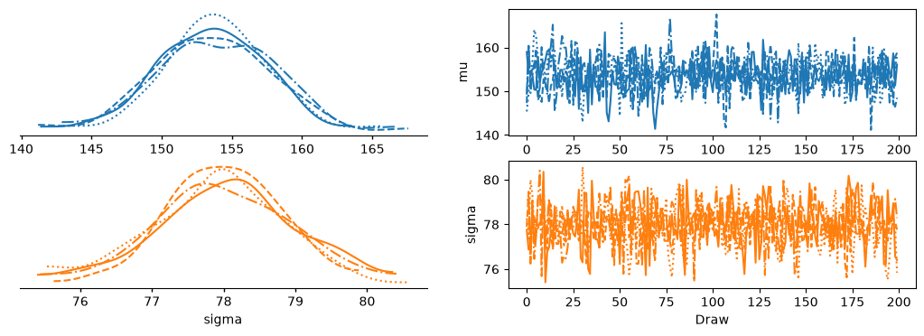
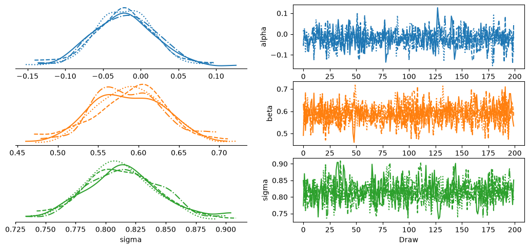
Tune the model using a Markov Chain Monte Carlo algorithm called Hamiltonian Monte Carlo (HMC), then plot the trace distribution.
def tune(model, tune=1000):
    """Tune the model and plot the trace distribution"""

    with model:
        # Normal model idata
        idata = pm.sample(200, tune=tune, random_seed=random_seed)

        # Plot the tuning/sampling
        az.plot_trace_dist(idata, kind='kde');
        plt.show()

        return idata
What the above optimization process is doing
At a high conceptual level, the frequency with which PyMC samples a point from the model is proportional to the likelihood of seeing that point. That’s the magic of MCMC.
How does this help us optimize the model on the observed data (the training data)? Because in determining the likelihood of seeing each parameter, the library uses the log-likelihood of the data under the given distribution.
Evaluating the model
Next, estimate the out of sample predictive accuracy, i.e., the performance on the test set. The leave-one-out estimate of the expected log pointwise density is defined as
\[elpd_{loo} = \sum_{i=1}^{n} \log p(y_i|y_{−i})\]where $y_{-i}$ is understood to be the data without the $i^{\text{th}}$ point.
This is calculated using az.loo below.
def evaluate(model, idata, x=None):
"""Evaluate the model"""
with model:
# Evaluate on the validation dataset
model.set_data('y', y_validation)
if x is not None:
model.set_data('x', x)
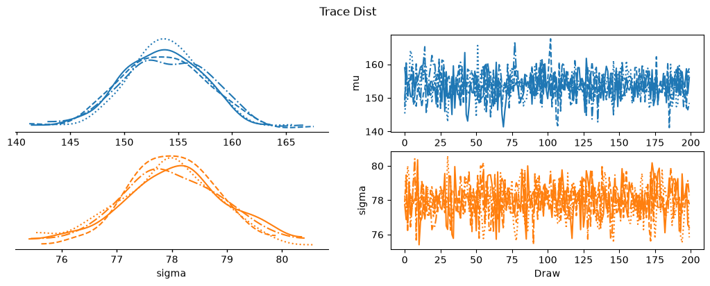
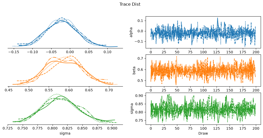
# Visually inspect the chains to check for convergence
plot_collection = az.plot_trace_dist(idata, kind='kde')
plot_collection.add_title('Trace Dist')
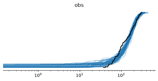
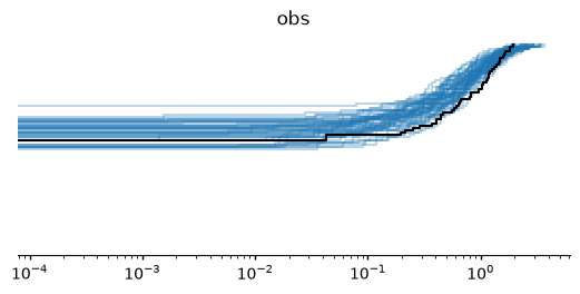
# Sample posterior predictive so that plot_ppc_dist will plot it
pm.sample_posterior_predictive(idata, extend_inferencedata=True, random_seed=random_seed)
# Observed distribution is black
plot_collection = az.plot_ppc_dist(idata)
axes = plot_collection.get_viz('plot')
axes.set_xscale('log')
# Leave-one-out cross validation of the log likelihood
pm.compute_log_likelihood(idata)
loo = az.loo(idata)
print('Leave-one-out cross-validation:')
print(loo)
idata = tune(normal_model, tune=1200)
evaluate(normal_model, idata)

# Present a summary of the specified variables
print('Summary:')
print(az.summary(idata, var_names=['mu', 'sigma']))
Initializing NUTS using jitter+adapt_diag...
Multiprocess sampling (4 chains in 4 jobs)
NUTS: [mu, sigma]


Sampling 4 chains for 1_200 tune and 200 draw iterations (4_800 + 800 draws total) took 1 seconds.
Sampling: [obs]
Leave-one-out cross-validation:
Computed from 800 posterior samples and 89 observations log-likelihood matrix.

         Estimate       SE
elpd_loo  -508.97     3.93
p_loo        0.20        -
------

Pareto k diagnostic values:
                         Count   Pct.
(-Inf, 0.66]   (good)       89  100.0%
   (0.66, 1]   (bad)         0    0.0%
    (1, Inf)   (very bad)    0    0.0%

Summary:
        mean    sd eti89_lb eti89_ub  ess_bulk  ess_tail r_hat mcse_mean  \
mu     153.7   3.9      150      160       739       625  1.01      0.14
sigma  77.98  0.92       76       79       739       535  1.00     0.034

      mcse_sd
mu       0.11
sigma   0.024
The $y$ distribution is long-tailed. I may be able to improve the fit if I take the square root of the target variable.
# Normalize y
def normalize(y):
    sqrt_y = np.sqrt(y)
    return (sqrt_y - np.mean(sqrt_y)) / np.std(sqrt_y)

y_train = normalize(y_train)
y_validation = normalize(y_validation)

# Plot a histogram showing how the target variable is distributed after transforming it
plt.hist(y_train)
plt.show()
I condition the posterior on one of the independent variables. I am somewhat trepid (or lazy, depending on your mood) in that I choose to use only a single column of X for conditioning initially.
I therefore perform feature selection by ranking the independent variables based on their correlation with the dependent variable. As a measure of correlation, I use Pearson’s r-coefficient.
# FEATURE SELECTION

# Compute Pearson's r-coefficient
rs = feature_selection.r_regression(X_train, y_train)
print("r-coefficient:")
print(rs)

# Choose the variable having the highest correlation with the target variable
i_greatest = np.argmax(np.abs(rs))
print()
print(f"Index of max r-coefficient is {i_greatest}")
x_train = X_train[:, i_greatest]
x_validation = X_validation[:, i_greatest]
print(f"Shape of x is {x_train.shape}")
r-coefficient:
[ 0.20352838  0.0023141   0.58700394  0.43448145  0.21197587  0.16948607
 -0.38990595  0.43074421  0.56174461  0.37991427]

Index of max r-coefficient is 2
Shape of x is (353,)
def linear_regression():
    """Build the computational graph for a linear regression model"""

    # Linear regression model to use the X
    with pm.Model() as model:

        x = pm.Data('x', x_train)
        y = pm.Data('y', y_train)

        # These priors are chosen because the data was standardized
        alpha = pm.Normal("alpha", mu=0, sigma=1)
        beta = pm.Normal("beta", mu=0.5, sigma=1)
        sigma = pm.HalfNormal("sigma", 1)

        # This represents a linear relationship between the dependent and independent variable
        obs = pm.Normal("obs", mu=alpha + beta * x, sigma=sigma, observed=y)

        return model
model = linear_regression()
idata = tune(model)
evaluate(model, idata, x_validation)
Initializing NUTS using jitter+adapt_diag...
Multiprocess sampling (4 chains in 4 jobs)
NUTS: [alpha, beta, sigma]


Sampling 4 chains for 1_000 tune and 200 draw iterations (4_000 + 800 draws total) took 1 seconds.
Sampling: [obs]


Leave-one-out cross-validation:
Computed from 800 posterior samples and 89 observations log-likelihood matrix.

         Estimate       SE
elpd_loo  -115.79     6.69
p_loo        0.83        -
------

Pareto k diagnostic values:
                         Count   Pct.
(-Inf, 0.66]   (good)       89  100.0%
   (0.66, 1]   (bad)         0    0.0%
    (1, Inf)   (very bad)    0    0.0%
print('Summary:')
print(az.summary(idata, var_names=['alpha', 'beta', 'sigma']))
Summary:
         mean     sd eti89_lb eti89_ub  ess_bulk  ess_tail r_hat mcse_mean  \
alpha  -0.022  0.041   -0.083    0.041      1168       631  1.00    0.0012
beta    0.589  0.045     0.52     0.66      1398       637  1.01    0.0012
sigma   0.814  0.032     0.76     0.86       908       616  1.00    0.0011

       mcse_sd
alpha  0.00091
beta   0.00081
sigma  0.00075
Bibliography
9.1. Toy datasets. (n.d.). Scikit-Learn. Retrieved June 17, 2026, from https://scikit-learn/stable/datasets/toy_dataset.html
Abril-Pla, O., Andreani, V., Carroll, C., Dong, L., Fonnesbeck, C. J., Kochurov, M., Kumar, R., Lao, J., Luhmann, C. C., Martin, O. A., Osthege, M., Vieira, R., Wiecki, T., & Zinkov, R. (2023). PyMC: A modern, and comprehensive probabilistic programming framework in Python. PeerJ Computer Science, 9, e1516. https://doi.org/10.7717/peerj-cs.1516
Vehtari, A., Gelman, A., & Gabry, J. (2017). Practical Bayesian model evaluation using leave-one-out cross-validation and WAIC. Statistics and Computing, 27(5), 1413–1432. https://doi.org/10.1007/s11222-016-9696-4